An Introduction to the Electronic Structure of Atoms and Molecules

    As either mass moves from one end of its line to the other, the potential energy (the energy which depends on the position of the mass) remains constant. We may set the potential energy equal to zero, and all the energy is then kinetic energy  (energy of motion). When the electron reaches the end of the line, we shall assume that it is reflected by some force. Thus at the ends of the line the potential energy rises abruptly to a very large value, so large that the electron can never "break through." We can plot potential energy versus position x along the line Fig. 2-1.

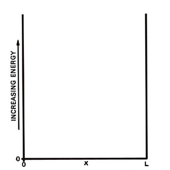Fig. 2-1. Potential energy diagram for a particle moving on a line of lenght L. When the electron  is at x = 0 or x = L the potential energy is infinite and for values of x between these limits (0< x < L ) the potential energy is zero.

We refer to the electron (or the particle of m = 1 g) as being in a potential well and we can imagine the abruptly rising potential at x = 0 and x = L to be the result of placing a "wall" at each end of the line. First, what are the predictions of classical mechanics regarding the energy of the mass of 1 g? The total energy is kinetic energy and is simply:
  We know from experience that u, the velocity, can have any possible value from zero up to very large values. Since all values for u are allowed, all values for E are allowed. We conclude that the energy of a classical system may have any one of a continuous range of values and may be changed by any arbitrary amount. Let us contrast with this conclusion the prediction which quantum mechanics makes regarding the energy of an electron in a corresponding situation.

    The quantum mechanical results are remarkable indeed, although they should not be surprising when we recall Bohr's explanation of the line spectra which are observed for atoms. Quantum mechanics predicts that there are only certain values of the energy which the electron confined to move on the line can possess. The energy of the electron is quantized. If this result could be observed for a massive particle, it would mean that only certain velocities were possible, say u = 1 cm/sec or 10 cm/sec but with no intermediate values! But then an electron is not really a particle. The expression for the allowed energies as given by quantum mechanics for this simple system is:
 

(1)

where again h is Planck's constant and n is an integer which may assume any value from one to infinity. Since only discrete values for E are possible, the appearance of the index n in equation (1) is necessary. A number such as n which appears in the expression for the energy is called a quantum number. Each value of the quantum number n fixes a value of E_n, one of the allowed energy values. We can indicate the possible values for the energy on an energy diagram. It is clear from equation (1) that for given values of m and L, E_n equals a constant (K = h²/8mL²) multiplied by n²:
 

(2)

Thus we can express the value of E_nin terms of so many units of K.

    Each line, called an energy level, in Fig. 2-2 denotes an allowed energy for the system and the figure is called an energy level diagram. Each level is identified by its value of n as a subscript. A corresponding diagram for the case of the classical particle would consist of an infinite number of lines with infinitesimally small spacings between them, indicating that the energy in a classical system may vary in a continuous manner and may assume any value. The energy continuum of classical mechanics is replaced by a discrete set of energy levels in quantum mechanics.

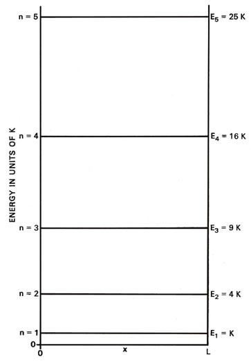Fig.  2-2.   Energy level diagram for an electron moving on a line of length L. Only the first few levels are shown.

Suppose we could give the electron sufficient energy to place it in one of the higher (excited) energy levels. Then when it "fell" back down to the lowest value of E (called the ground level, E₁), a photon would be emitted. The energy e of the photon would be given by the difference in the values of E_n and E₁ and, since e = hv the frequency of the photon would be given by the relationship:
  which is Bohr's frequency condition (I-4). Thus only certain frequencies would be emitted and the spectrum would consist of a series of lines.

    We can illustrate the change in energy when the electron falls to the lowest energy level by connecting the upper level and the n = 1 level by an  arrow in an energy level diagram. The frequency of the photon emitted during the indicated drop in energy is proportional to the length of the arrow, i.e., to the change in energy (Fig. 2-3). The line directly beneath each arrow represents the value of the frequency for that drop in energy. Since the differences in the lengths of the arrows increase as n increases, the  separations between the observed frequencies show a corresponding increase. The spectrum, therefore, consists of a series of lines, with the spacings between the lines increasing as n increases. If the energy was not quantized and all values were possible, all jumps in energy would be possible and all frequencies would appear. Thus a continuum of possible energy values will produce a continuous spectrum of frequencies. A line spectrum, on the other hand, is a direct manifestation of the quantization of energy.

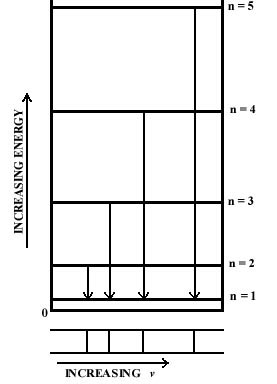Fig. 2-3.  The origin of a line spectra.

    In the quantum case, as in the classical case, all of the energy will be in the form of kinetic energy. We may obtain an expression for the momentum of the electron by equating the total value of the energy E_n to p²/2m, where p is the momentum
(= mu) of the electron, (p²/2m is another way of expressing 2mu².)
  This gives:
  A plus and a minus sign must be placed in front of the number which gives the magnitude of the momentum to indicate that we do not know and cannot determine the direction of the motion. If the electron moves from left to right the sign will be positive. If it moves from right to left the sign will be negative. The most we can know about the momentum itself is its average value. This value will clearly be zero because of the equal probability for motion in either direction. The average value of p², however, is finite.

    Since the lowest allowed value of the quantum number n in the quantum mechanical expression for the energy is unity, it is evident that the energy can never equal zero. A confined electron can never be motionless. The expression for E_n also indicates that the kinetic energy and the momentum increase as the length of the line L is decreased. Thus the kinetic energy and momentum of the electron increase as its motion becomes more confined. This is both an important and a general result and will be referred to again.