An Introduction to the Electronic Structure of Atoms and Molecules

    The concept of a trajectory is fundamental to classical mechanics. Given a particular mass with a given initial velocity and a knowledge of the forces acting on it, we may use classical mechanics to predict the exact position and velocity of the particle at any future time. Thus we speak of the trajectory of the particle and we may calculate it to any desired degree of accuracy. It is also possible, within the framework of classical mechanics, to measure the position and velocity of a particle at any given instant of time. Thus classical mechanics correctly predicts what one can experimentally measure for massive particles.

    We have previously mentioned the difficulties which are encountered when we attempt to determine the position of an electron. The results of the Compton effect indicate that part of the energy of the photon used in making the observation is transferred to the electron, and we invariably disturb the electron when we attempt to measure its position. Thus it is not surprising to find that quantum mechanics does not predict the position of an electron exactly. Rather, it provides only a probability as to where the electron will be found. When we consider the experiments which attempt to define the position of the electron, we shall find that this is the maximum information that can indeed be obtained even experimentally. The new mechanics again predicts only what can indeed be measured experimentally.  We shall illustrate the probability aspect in terms of the system of an electron confined to motion along a line of length L. Quantum mechanical probabilities are expressed in terms of a distribution function which in this particular case we shall label P_n(x).

    Consider the line of length L to be divided into a large number of very small segments, each of length Dx. Then the probability that the electron is in one particular small segment Dx of the line is given by the product of Dx and the value of the probability distribution function P_n(x) for that interval. For example, the probability distribution function for the electron when it is in the lowest energy level, n = 1, is given by P₁(x) (Fig. 2-4).

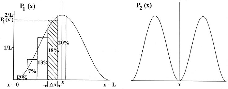
The probability that the electron will be in the particular small interval Dx indicated in Fig. 2-4 is equal to the shaded area, an area which in turn is equal to the product of Dx and the average value of P₁(x) throughout the interval Dx, called P₁(x'),
      The curve P₁(x) may be determined in the following manner. We design an experiment able to determine whether or not the electron is in one particular segment Dx of the line when it is known to be in the quantum level n = 1. (One way in which this might be done is described below.) We perform the experiment a large number of times, say one hundred, for each segment and record the ratio of the number of times the electron is found in a particular segment to the total number of observations made for that segment. For example, an electron is found to be in the segment marked Dx (of length 0.1 L) in the figure for P₁(x) in 18 out of 100 observations, or 18% of the time. In the other 82 observations the electron was in one of the other segments. Thus the average value of P₁(x) for this segment, called P₁(x') must be 1.8/L since P₁(x')Dx  = (1.8/L) (0.1 L) = 0.18 or 18%. A similar set of experiments is made for each of the segments Dx and in each case a rectangle is constructed with Dx as base and with a height equal to P₁(x) such that the product P₁(x)Dx equals the fractional number of times the electron is found in the segment Dx. The limiting case in which the total length L is divided into a very large number of very small segments (Dx ® dx) would result in the smooth curve shown in the figure for P₁(x).

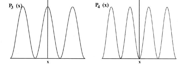
    There is a different probability distribution for each value of E_n, or each quantum level, as shown, for example, by the probability distributions for the energy levels with n = 2, 3, 4, 5 and 6 (Fig. 2-4).  The probability of finding the electron at the positions where the curve touches the x-axis is zero. Such a zero is termed a node. The number of nodes is always n-1 if we do not count the nodes at the ends of each P_n(x) curve.

    Let us first contrast these results, particularly that for P₁(x), with the corresponding classical case. Since a classical analysis allows us to determine the position of a particle uniquely at any instant, either theoretically or experimentally, the idea of a probability distribution is foreign to a classical mechanical analysis. However, we still can determine the classical probability distribution for the particle confined to motion on a line. Since there are no forces acting on the particle as it traverses the line, it will be equally likely to be found at any point on the line (Fig 2-5). This probability will be the same regardless of the energy. There is again a striking difference between the classical and the quantum mechanics results. For the first quantum level, the graph of P₁(x) indicates the electron will most likely be found at the midpoint of the line. Furthermore, the form of P_n(x) changes with every change in energy. Every allowed value of the of the energy has associated with it a distinct probability distribution for the electron.  Theses are the predictions of quantum mechanics regarding the position of a bound electron. Now let us investigate the experimental aspect of the problem to gain some physical reason for these predictions.

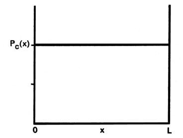Fig. 2-5. The classical probability distribution for motion on a line. This is the result obtained when the particle is located a large number of times at random time intervals. The classical probability function Pc(x) is the same for all values of x and equals 1/L, i.e., the particle is equally likely to be found at any value of x between 0 and L

(3)

Fig. 2-6. An idealized experiment for detecting he position of an electron.

  Remembering the Compton effect and bearing in mind that we wish to disturb the electron as little as possible during the observation, we shall inquire as to the results obtained when a single photon is scattered from the electron. A single photon will not yield the complete diffraction pattern at A, but will instead produce a single flash of light. A diffraction pattern is the result of many photons passing through the microscope and represents the probability distribution for the emergent photons when they have been scattered by an electron lying between x' and x''. A single photon, when scattered from an electron within the length Dx, is however still diffracted and will produce a flash of light somewhere in one of the areas defined by the probability distribution produced by many photons passing through the system.

  Thus even when we use but a single photon in our apparatus the uncertainty Dx in our experimentally determined position of the electron will still be given by equation (3). Obviously, if we want to locate an electron which is confined to move on a line to within a length that is small compared to the length of the line, we must use light which has a wavelength much less than L. This is exactly what equation (3) states: the shorter the wavelength of the light which is used to observe the electron, the smaller will be the uncertainty Dx. That being the case, why not do the experiment with light of very short wavelength compared to the length L, say l = (1/100)L? Then we can hope to find the electron on one small segment of the line, each segment being approximately (1/100)L in length. Let us calculate the frequency and energy of a photon which has the required wavelength of l = (1/100)L. As before, we set L equal to a typical atomic dimension of 1 x 10^-8 cm.
  We are immediately in difficulty, because the energy of the electron in the first quantum level is easily found to be:
  The energy of the photon is approximately 1 x 10⁴ times greater than the energy of the electron! We know from the Compton effect that the collision of a photon with an electron imparts energy to the electron. Thus the electron after the collision will certainly not be in the state n = 1. It will be excited to oneCwe don't know whichCof the excited levels with n = 2 (E = 4K) or n = 3 (E = 9K), etc. The result is clear. If we demand an intimate knowledge of what the position of the electron is in a given state, we can obtain this information only at the expense of imparting to the electron an unknown amount of energy which destroys the system, i.e., the electron is no longer in the n = 1 level but in one of the other excited levels. If this experiment was repeated a large number of times and a record kept of the number of times an electron was located in each segment of the line (roughly (1/100)L), a probability plot similar to Fig. 2-4 would be obtained.

    We can ask another kind of question regarding the position of the electron: "How much information can be obtained about the position of the electron in a given quantum level without at the same time destroying that level?" The electron cannot accept energy in an amount less than that necessary to excite it to the next quantum level, n = 2. The difference in energy between E₂, and E₁, is 3K. Thus if we are to leave the electron in a state of known energy and momentum we must use light whose photons possess an energy less than 3K.

   Let us calculate the wavelength of the light with e = 2K and compare this value with the length L.
      The wavelength is greater than the length of the line L. From equation (3) it is clear that the uncertainty in the position of the particle will be of the order of magnitude of, or greater than, L itself. The electron will appear to be blurred over the complete length of the line in a single experiment! Thus there are two interpretations which can be given to the probability distributions, depending on the experiment which is performed. The first is that of a true probability of finding the electron in a given small segment of the line using light of very short l relative to L. This experiment excites the electron, changes the system and leaves the electron with an unknown amount of energy and momentum. We have destroyed the object of our investigation. We now know where it was in a given experiment but not where it will be, in terms of energy or position.

   Alternatively, we could use light with a l approximately equal to L. This does not excite the electron and leaves it in a known energy level. However, now the knowledge of the position is very uncertain. The photons are scattered from the system and give us directly the smeared distribution P₁ pictured in Fig. 2-4. In a real sense we must accept the fact that when the electron remains in a given state it is "smeared out" and "looks like" the pictures given for P_n. Thus we can interpret the P_n's as instantaneous pictures of the electron when it is bound in a known state, and forgot their probability aspect. This "smeared out" distribution is given a special name; it is called the electron density distribution. There will be a certain fraction of the total electronic charge at each point on the line, and when we consider a system in three dimensions, there will be a certain fraction of the total electronic charge in every small volume of space. Hence it is given the name electron density, the amount of charge per unit volume of space. The P_n's represent a charge density distribution which is considered static as long as the electron remains in the nth quantum level. Thus the P_n functions tell us either (a) the fraction of time the electron is at each point on the line for observations employing light of short wavelength, or (b) they tell us the fraction of the total charge found at each point on the line (the whole of the charge being spread out) when the observations are made with light of relatively long wavelength.

   The electron density distributions of atoms, molecules or ions in a crystal can be determined experimentally by X-ray scattering experiments since X-rays can be generated with wavelengths of the same order of magnitude as atomic diameters (1 ´ 10^-8 cm). In X-ray scattering the intensity of the scattered beam and the angle through which it is scattered are measured. The distribution of negative charge within the crystal scatters the X-rays and determines the intensity and angle of scattering. Thus these experimental quantities can be used to calculate the form of the electron density distribution.

    There is a definite quantum mechanical relationship governing the magnitudes of the uncertainties encountered in measurements on the atomic level. We can illustrate this relationship for the one-dimensional system. Let us consider the minimum uncertainty in our observations of the position and the momentum of the electron moving on a line obtained in an experiment which leaves the particle bound in a given quantum level, say n = 1. This will require the use of light with l ~ L. We have seen that the use of light of this wavelength limits us to stating that the electron is somewhere on the line of length L. We can say no more than this with certainty unless we use light of much shorter l , and then we will change the quantum number of the electron. The uncertainty in the value of the position coordinate, which we shall call Dx, is just L, the length of the line:
  We have previously shown that the momentum of the electron in the nth quantum level is given by:
  the plus and minus signs denoting the fact that while we know the magnitude of the momentum we cannot determine whether the electron is moving from left to right (+nh/2L) or from right to left (-nh/2L). The minimum uncertainty in our knowledge of the momentum is the difference between these two possibilities, or for n = 1:
  The product of the uncertainties in the position and the momentum is:
  This result is a particular example of a general relationship governing the product of the uncertainties in the momentum and position known as Heisenberg's uncertainty principle. In the general case, the equality sign in the above equation is replaced by the symbol "³" which denotes that the product in the uncertainties DpDx equals or exceeds the value of Planck's contant h, that is, the general statement is given by DpDx ³ h.

    If we endeavour to decrease the uncertainty in the position coordinate (i.e., make D x small) there will be a corresponding increase in the uncertainty of the momentum of the electron along the same coordinate, such that the product of the two uncertainties is always equal to Planck's constant. We saw this effect in our experiments wherein we employed light of short l to locate the position of the electron more precisely. When we did this we excited the electron to one of the other available quantum states, thus making a knowledge of the energy and hence the momentum uncertain. We might also try to defeat Heisenberg's uncertainty principle by decreasing the length of the line L. By shortening L, we would decrease the uncertainty as to where the electron is. However, as was noted previously, the momentum increases as L is decreased and the uncertainty in p is always the same order of magnitude as p itself; in this case twice the magnitude of  p. Thus the decrease in Dx obtained by decreasing L is offset by the increase in Dp which accompanies the increased confinement of the electron; the product DxD p remains unchanged in value.

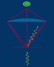
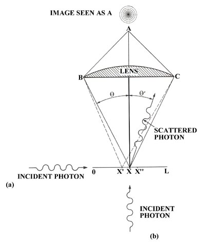
    We can illustrate the operation of Heisenberg's uncertainty principle for a free particle by referring again to our hypothetical experiment in which we attempted to locate the position of an electron by using a microscope. We imagine the electron to be free and travelling with a known momentum in the direction of the x-axis with a photon entering from below along the y-axis. When the photon is scattered by the electron it may transfer momentum to the electron and continue on a line which makes an angle q' to the y-axis (Fig. 2-6). The photon, in doing so, will acquire momentum in the direction of the x-axis, a direction in which it initially had none. Since momentum must be conserved, the electron will receive a recoil momentum, a momentum equal in magnitude but opposite in direction to that gained by the photon. This is the Compton effect. Thus our act of observing the electron will lead to an uncertainty in its momentum as the amount of momentum transferred during the collision is uncontrollable. We may, however, set limits on the amount transferred and in this way determine the uncertainty introduced into the value of the momentum of the electron.

    The momentum of the photon before the collision is all directed along the y-axis and has a magnitude equal to h/l . After colliding with the electron the photon may be scattered to the left or to the right of the y-axis through any angle q' lying between 0 and q and still be collected by the lens of the microscope and seen by the observer at A. Thus every photon which passes through the microscope will have an uncertainty of 2(h/l)sinq in its component of momentum along the x-axis since it may have been scattered by the maximum amount to the left and acquired a component of -(h/l)sinq or, on the other hand, it may have been scattered by the maximum amount to the right and acquired a momentum component of +(h/l)sinq. Any x-component of momentum acquired by the photon must have been lost by the electron and the uncertainty introduced into the momentum of the electron by the observation is also equal to 2(h/l)sinq .

    In addition to the uncertainty induced in the momentum of the electron by the act of measurement, there is also an inherent uncertainty in its position (equation (3)) because of the limited resolving power of the microscope. The product of the two uncertainties at the instant of measurement or immediately following it is:
  Heisenberg's uncertainty relationship is again fulfilled. Our experiment employs only a single photon which, since light itself is quantized, represents the smallest packet of energy and momentum which we can use in making the observation. Even in this idealized experiment the act of observation creates an unavoidable disturbance in the system.